1 音に関する単位変換など

1.1 音速

空気中の音速は、気温を$T$（℃）としたとき$331.5 + 0.6T$で計算できます。そのままプログラムにしたのが以下です。気温を指定しない場合は、東京の平均気温である16.3度を使用します。

"""
    speed_of_sound([t])

Compute speed of sound in air from specified temperature `t` degrees
(celcius).

If you do not provide `t` the default value used is 16.3 which is the
average temperature in Tokyo).

# Examples
“`julia-repl
julia> speed_of_sound()
341.28

julia> speed_of_sound(20)
343.5
“`
"""
function speed_of_sound(temperature=16.3)
  331.5 + 0.60 * temperature
end

【使い方】気温20度のときの音速は？

julia> speed_of_sound(20.0)
343.5

343.5 m/sでした。

1.2 周波数と音高にかかわるもの

1.2.1 MIDIセント

MIDIセント値は、MIDIノート番号とそこからのずれを同時に扱うことができる便利な方法です。たとえば、中央のドはMIDIノート番号で60で、そこから15セント上のピッチは、60×100＋15＝6015と表せます。

"""
    freq_to_midicent(freq[, concert_pitch=440])

Convert frequency (Hz) to MIDI cent value (MIDI note number times 100
for representing partial pitch).

# Examples
“`julia-repl
julia> freq_to_midicent(1000)
8321.309485364913

julia> freq_to_midicent(1000, 442)
8313.458070324787
“`
"""
function freq_to_midicent(freq, concert_pitch=440)
  log2(freq / concert_pitch) * 1200 + 6900
end

"""
Convert MIDI cent value (MIDI note number times 100 for representing
partial pitch) to frequency (Hz).
"""
function midicent_to_freq(midicent, concert_pitch=440)
  concert_pitch * 2^((midicent - 6900) / 1200)
end

【使い方】コンサートピッチが442 Hzのとき、ピアノ鍵盤上で1000 Hzはどのあたり？

julia> freq_to_midicent(1000, 442)
8313.4580703247866

MIDIノート番号で83番付近。ピッタリより若干（13.458セント）上。

オクターブ番号を知りたいときもあります。オクターブ番号とは、中央のド（約262 Hz）をC4としたときの「4」です。MIDIセントの計算を元に以下のようにしてみました。小数点以下を切り捨てればオクターブ番号となります。

"""
    freq_to_octave(freq[, concert_pitch=440])

Convert frequency (Hz) to standard octave number (center C = 4).

# Examples
“`julia-repl
julia> freq_to_octave(1000)
5.934424571137427

julia> freq_to_octave(262.815, 442)
4.0000012493009365
“`
"""
function freq_to_octave(freq, concert_pitch=440)
    freq_to_midicent(freq, concert_pitch) / 1200 - 1;
end

1.2.2 臨界帯域

臨界帯域についての計算式はZwicker and Terhardt (1980)によるものもありますが、ここではTraunmllerの「Analytical Expressions for the Tonotopic Sensory Scale」(J. Acoust. Soc. Am., 1990, https://doi.org/10.1121/1.399849)に記載されている数式を参考にしました。

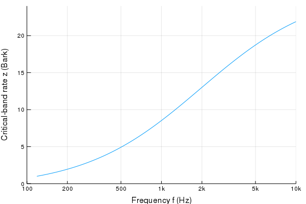
まずは、周波数を臨界帯域番号（critical band rate）に直すもの。だいたい200 Hz〜6700 Hzの範囲でZwickerのBark尺度と合致するということです。

"""
freq_to_bark(freq)

Convert frequency value (Hz) to critical band rate (bark)
"""
function freq_to_bark(freq)
  z = ((26.81 * freq) / (1960 + freq)) - 0.53;
  if z < 2
    z += 0.15 * (2 - z);
  elseif z > 20.1
    z += 0.22 * (z - 20.1);
  end
  return(z);
end

その逆に、臨界帯域番号を周波数に直すもの。

"""
    bark_to_freq(z)

Calculate critical band rate (in Hz) at britical band rate z (in bark).
"""
function bark_to_freq(z)
  1960 / (26.81 / (z + 0.53) - 1);
end

たとえば、以下のプログラムでは周波数と臨界帯域番号の関係を図示するグラフ（図）を作成します。Traunmller (1990)のFig.2に相当します。

using Plots
b = 1 : 0.1 : 24;
plot(bark_to_freq.(b), b, legend=false,
     xscale=:log10, xlim=(100, 10000), ylim=(0,24),
     xlabel="Frequency f (Hz)",
     xticks=([100, 200, 500, 1000, 2000, 5000, 10000],
             ["100", "200", "500", "1k", "2k", "5k", "10k"]),
     ylabel="Critical-band rate z (Bark)")

図: 周波数（横軸）と臨界帯域番号（縦軸）の関係

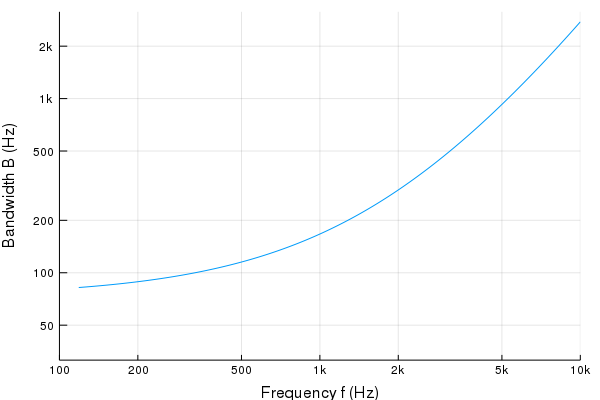
また、それぞれの臨界帯域の周波数幅をHz単位で出すものは以下のようになります。

"""
    bark_to_bandwidth(z)

Calculate critical bandwidth (in Hz) at critical band rate z (in bark).
"""
function bark_to_bandwidth(z)
  B = 52548 / (z^2 - 52.56z + 690.39);
  return(B);
end

こちらも同様に周波数と臨界帯域幅の関係を図示するグラフ（図）が作れます。Traunmller (1990)のFig.1に相当します。

図: 周波数（横軸）と臨界帯域幅（縦軸）の関係

1.3 音圧と振幅にかかわるもの

1.3.1 デシベル値から振幅を計算する

波形の振幅（音圧に比例）を$p$、その基準値を$p_0$としたときに、デシベル値との対応は次のようになっています。

$$L = 10\log_{10}\frac{p^2}{p_0^2}$$ (1)

$$~ = 10\log_{10}\left(\frac{p}{p_0}\right)^2$$ (2)

$$~ = 20\log_{10}\frac{p}{p_0}$$ (3)

$$p = 10^\frac{L}{20} \cdot p_0$$ (4)

デシベル値の計算には基準値が必要になりますが、以下のプログラムでは基準値（base）をデフォルトで1としています。

"""
Calculate amplitude value from dB value.
"""
function db_to_amplitude(db_value, base=1.0)
  10 ^ (db_value / 20) * base
end

baseの値を指定することで、適切なdB値を求めることができます。たとえば音圧レベルの計算には $p_0=20\times 10^{-6}$を使いますので、

julia> db_to_amplitude(94, 20e-6)
1.0023744672545452

のように $94\,\mathrm{dB}\approx 1\,\mathrm{Pa}$と計算できます。

1.3.2 振幅からデシベル値を計算する

"""
Calculate dB value from amplitude value.
"""
function amplitude_to_db(amp_value, base=1.0)
  20 * log10(amp_value / base)
end

1.3.3 デシベル値からパワーを計算する

"""
Calculate power value from dB value.
"""
function db_to_power(db_value, base=1.0)
  10^(db_value / 10) * base
end

1.3.4 パワーからデシベル値を計算する

"""
Calculate dB value from power value.
"""
function power_to_db(pow_value, base=1.0)
  10*math.log10(pow_value / base)
end

1.3.5 RMS（実効値）

"""
`rms(x)` computes root-mean-square of a signal `x`.
"""
function rms(x)
  sqrt(sum(x .^ 2.0) / length(x))
end

rms()はDSP.jlに含まれているので必要ないかもです。

"""
adjust signal level to be the target
"""
function rms_match(x, target_rms)
  x * db_to_amplitude(target_rms - amplitude_to_db(rms(x)))
end

"""
Calculate RMS of a signal as in moving average.

Usage:
    using LibSndFile
    snd = load("audio.wav")
    (t,r) = rms_moving(snd, window_size=8192, hop_size=1024)
    using PyPlot
    plot(t, r)
"""
function rms_moving(snd, window_size=8192, hop_size=1024)
  x = snd.data;
  fs = snd.samplerate;
  num_frames = floor((length(x) + window_size-1) / hop_size)
  xx = [x ; zeros(typeof(x[1]), 2 * window_size)]
  rmss = zeros(num_frames)
  for n=0:num_frames-1
    xxx = xx[Int(hop_size*n+1) : Int(hop_size*n+window_size)]
    rmss[Int(n+1)] = rms(xxx)
  end
  t = (0:num_frames-1) * hop_size
  return(t, rmss)
end

1.3.6 クレストファクター

function crest_factor(x)
  return(maximum(abs.(x)) / rms(x))
end

1.4 時間にかかわるもの

"""
Convert time (in seconds) to number of samples.
"""
function time_to_samples(sec, samprate=44100)
  sec * samprate
end

"""
Convert number of samples to time (in seconds).
"""
function samples_to_time(samples, samprate=44100)
  samples / samprate
end